I’d start with a simple statistical detector and move up only when replay tests show it misses the anomalies you need to catch. Compare all 5 model families on latency, memory, drift response, interpretability, and maintenance - not scoring speed alone.
My shortlist: statistics for simple spikes, online trees for nonlinear feature patterns, projection/sketch/density methods for compact state or local outliers, RRCF for bounded sample storage, and neural detectors when sequence context matters.
Quick Comparison
| Model family | Latency | Memory | Drift response | Interpretability | Maintenance |
|---|---|---|---|---|---|
| Incremental statistics | Very low | Minimal to low | Windows update baselines | Clear thresholds | Low |
| Online tree ensembles | Low scoring; updates vary | Depends on tree count and depth | Online updates or retraining | Less direct than statistics | Moderate |
| Projection, sketch, and streaming density | Low for sketches; window-dependent for density | Compact sketches; larger density windows | Summary or reference updates | Neighbor scores are easier to explain than sketches | Moderate to high |
| Random Cut Forests (RRCF) | Low to medium | Capped by samples and trees | Update policy matters; shifts may need resets | Cut and path details | Moderate |
| Neural detectors | Higher; workload-dependent | High | Memory updates or retraining | Harder to explain | High |
Fast scoring is only part of the test. I’d measure p50 and p99 score-plus-update latency, peak memory, detection delay, and false alarms per hour using time-ordered replay.
My final rule: <u>reject models that exceed your production limits</u>, then choose the one your team can explain, tune, and support.
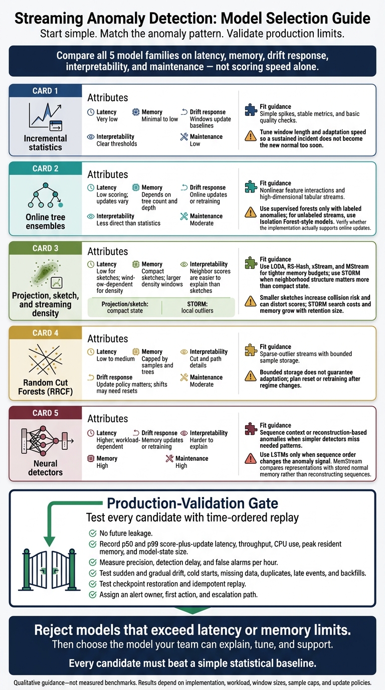
Streaming Anomaly Detection: Model Selection Guide
1. Incremental Statistical Detectors
Scoring and Update Latency
Moving averages, EWMA, and rolling z-scores score data in near-constant time [3]. But fast scoring helps only if updates stay cheap. Measure scoring, updates, and refits separately: fast predictions don't mean low maintenance costs. For Holt-Winters, ARIMA-style residual monitoring, and robust Kalman filters, check whether the implementation updates state incrementally or needs a refit.
Memory Use
Windowed detectors retain only aggregates or recent observations [3]. Holt-Winters, ARIMA, and Kalman variants may hold more state, so measure retained state separately from update cost.
History depth matters most for seasonal signals. Many statistical detectors need months of data to build a stable baseline. Seasonal workloads may need a full year [7].
Response to Concept Drift
Z-scores and IQR rules work well for isolated spikes. Moving averages, EWMA, and ARIMA-style residual monitoring are better suited to sustained level shifts [6]. Tune window length and adaptation speed so a sustained incident doesn't reset the baseline too soon [2].
For seasonal deviations, test Holt-Winters or seasonal ARIMA against the expected cycle. Check that your history covers the cycle you're evaluating [7].
Interpretability and Maintenance
Z-scores and IQR are easy to interpret because their rules are explicit [6]. Thresholds still need calibration, and static thresholds can be rigid when conditions change [1]. A 2-standard-deviation threshold is a starting point, not a guarantee of a low false-alert rate [7].
Assign alert owners and response steps before launch. Revisit thresholds and refit plans after major process changes [7]. When drift or nonlinearity exceeds what fixed thresholds can handle, online tree ensembles are the next step.
sbb-itb-bec6a7e
Real-time anomaly detection on streaming data using Random Cut Forest on Apache Flink
2. Online Tree Ensembles
Tree ensembles handle nonlinear patterns and previously unseen anomalies better than incremental statistics, without rigid per-feature thresholds [1][4]. Use supervised forests only when you have labeled anomalies. For unlabeled streams, use Isolation Forest-style models [1][4]. These gains matter only if production update costs stay low.
Scoring and Update Latency
Scoring is usually fast. Update latency, though, depends on whether the implementation supports true online updates or requires batch retraining. Benchmark scoring and updates separately against your live traffic pattern - fast predictions can mask costly retraining.
Memory Use
Tree ensembles generally need more memory than simple statistical baselines. Measure peak memory use during updates and retraining, accounting for tree count and depth. A small memory footprint doesn't help if the model can't absorb new behavior fast enough.
Response to Concept Drift
Drift response depends on how fast the model learns new baselines without treating true anomalies as normal. Controlled online updates or retraining can help it adjust better than static models [2]. But faster adjustment can add tuning and retraining work while making alert thresholds less stable.
Interpretability and Maintenance
Tree ensembles are generally easier to interpret than neural networks [4], but they're less transparent and need more maintenance than simple statistical detectors. Calibrate thresholds against reviewed alerts and your team's response capacity to limit false alerts [7]. Maintenance usually includes scheduled retraining and retraining after major process changes [7].
3. Projection, Sketch, and Streaming Density Detectors
Use LODA, RS-Hash, xStream, and MStream for tighter memory budgets; use STORM when neighborhood structure matters more than compact state. When tree ensembles become too heavy for live state updates, these detectors trade some fidelity for lower memory use and faster scoring. The first group compresses state through projections, hashes, or sketches. STORM keeps a sliding window and scores neighborhoods.
Scoring and Update Latency
Projection- and sketch-based methods avoid full-window scans, so they score faster than neighborhood-based methods. STORM searches stored observations, which means its update cost grows with window size [3][8].
Memory Use
RS-Hash and MStream cut memory use, but smaller sketches increase collision risk and can distort scores. LODA, xStream, and STORM retain more state. STORM’s memory use grows directly with retention size [3][8]. These memory choices also affect how quickly each method forgets old behavior.
Response to Concept Drift
The right fit depends on feature structure and baseline behavior, not just the stream label [1][2][8]. Shorter sliding or tumbling windows respond faster to drift; longer windows favor stability [2][3]. More aggressive adaptation makes it harder to explain why a point was flagged.
Interpretability and Maintenance
STORM is easier to explain: it flags points with too few nearby neighbors. Projection- and sketch-based methods are harder to audit because their scores are less transparent. STORM still needs careful distance-metric selection and feature scaling. Normalize numeric inputs and encode categorical values consistently before scoring [6][7].
4. Random Cut Forests (RRCF)
Scoring and Update Latency
RRCF isolates sparse points in a tree forest and caps stored state for streaming use [1][6]. More trees and larger samples increase latency. Benchmark scoring and updates separately under production load.
Memory Use
Sample size and tree count set RRCF’s memory limits [6]. Set both caps before deployment, then test whether added capacity improves detection. RRCF sits between forests that require frequent retraining and sketch-based detectors. Latency and maintenance needs depend on the implementation.
Response to Concept Drift
Bounded storage doesn’t guarantee that RRCF will adjust to changing data. Plan a reset or retrain after regime changes, and review that decision on a fixed schedule [7].
Interpretability and Maintenance
RRCF can be easier to explain than neural methods, but stable production use still requires alert feedback and tuning. Use explainability tools [2], review and label false positives [7], tier alerts by business impact [5], and give 1 owner responsibility for tuning [7]. Move to neural detectors if anomalies depend on sequence context or reconstruction error.
5. Neural Sequence, Reconstruction, and Memory-Based Detectors
Neural models offer more temporal context at a higher cost. Use them when simpler detectors miss sequence patterns. They are the highest-complexity option in this comparison.
Autoencoders reconstruct inputs and flag anomalies when reconstruction error increases. LSTM autoencoders also model sequences and track long-range temporal dependencies, but they require ordered windows and more memory. Both train only on normal data and need clean normal baselines [1][2][6]. MemStream instead compares incoming representations with stored normal memory rather than reconstructing sequences [1][2].
Scoring and Update Latency
Measure inference latency separately from training and baseline setup. Neural models can score inputs in under 100 ms in production, while initial data processing and baseline setup typically take 1-2 weeks [2][5]. LSTMs add processing work for temporal windows. MemStream also updates its normal memory over time [1][2].
Memory Use
Budget for model weights, feature processing, and sliding-window buffers for LSTMs or stored normal states for MemStream [1][2]. Historical training data adds a separate storage cost. Plan for at least 30 days of raw logs, or 90 days if you need seasonal coverage [5]. Match retention to the patterns your detector needs to learn.
Response to Concept Drift
Autoencoders need periodic retraining or adaptive updates as normal behavior changes [2][7]. MemStream updates its normal memory over time [2]. Schedule retraining at fixed intervals or after major process changes [7].
Interpretability and Maintenance
Reconstruction error and memory-based scores can show that a threshold fired, but neural detectors remain harder to interpret than statistical methods [1][6]. Maintenance demands are also high: teams must monitor data quality, tune sensitivity, and manage retraining [7].
Use LSTMs only when sequence order changes the anomaly signal. Their gains come with higher operating costs, which the next section compares directly with production limits.
Compare Latency, Memory, Drift, and Maintenance
Test all 5 model families under the same workload, memory limits, and drift conditions to see which fit your production constraints.
Scoring and Update Latency
Measure end-to-end latency, not scoring time alone. Track score time, update time, and alert delay separately under matched workloads [3]. Use replay to test dropouts, noise, late events, and alert load [3][7].
| Model family | Relative latency | Best fit |
|---|---|---|
| Incremental statistical detectors | Ultra-low | Low-variance streams with stable seasonality; static thresholds can struggle when conditions change [1][6] |
| Online tree ensembles | Low | High-dimensional tabular data [6] |
| Projection, sketch, and streaming density methods | Medium | High-dimensional streams with sparse anomalies [4] |
| Random Cut Forests (RRCF) | Low to medium | Sparse-outlier streams with bounded state |
| Neural detectors | High | Complex sequence patterns; transformers can reduce inference latency, but memory use and interpretability carry high costs [1][2][4] |
Fast scoring won't help if growing state pushes the model past deployment limits.
Memory Use
Measure peak resident memory and serialized model-state size separately [3]. Cap entities and categories so state cannot grow without limits.
| Model family | Retained state | Memory profile |
|---|---|---|
| Incremental statistical detectors | Recursive statistics or windows | Minimal to low |
| Online tree ensembles | Trees and retained samples | Low |
| Projection, sketch, and streaming density methods | Summaries or reference samples and search structures | Usually bounded for sketches; medium for density methods |
| Random Cut Forests (RRCF) | Trees and sample caps | Low to medium |
| Neural detectors | Weights, context, and stored representations | High |
Response to Concept Drift
Separate built-in adaptation from retraining managed by operators. Test sudden shifts and gradual changes separately, then compare recovery time, false alarms, and missed detections [2][7].
| Model family | Drift response | Adaptation controls | Main failure mode |
|---|---|---|---|
| Incremental statistical detectors | Rebaselining with windows | Window limits and threshold updates | Static thresholds lag change |
| Online tree ensembles | Recalibration or replacement, if supported | Update schedule | Batch retrains lag change |
| Projection, sketch, and streaming density methods | Summary updates or reference replacement | Recalibration and update rules | Summaries or references go stale |
| Random Cut Forests (RRCF) | Reset or retrain after regime change | Reset triggers and update schedule | Stale cuts after distribution shift |
| Neural detectors | Adaptive updates, replay, or retraining | Update triggers and replay policy | Forgetting, contamination, or delayed feedback [2] |
The team must be able to tune and support adaptation in production for it to help.
Interpretability and Maintenance
An explanation does not prove root cause. Statistical thresholds are easier to inspect than neural scores [1][6].
| Model family | Explanation artifacts | Tuning burden | Maintenance risks |
|---|---|---|---|
| Incremental statistical detectors | Residuals and thresholds | Low | Poor seasonal calibration |
| Online tree ensembles | Decision paths | Moderate | Stale trees or feature changes |
| Projection, sketch, and streaming density methods | Bins, hash buckets, or neighbor references | Moderate to high | Collisions, limited investigation detail, or contaminated references |
| Random Cut Forests (RRCF) | Path/cut structure | Moderate | Update timing and sample cap drift |
| Neural detectors | Feature-level errors or memory references | High | Version mismatch and difficult rollback |
Deployment checklist:
- Validate time-ordered replay with no future leakage. Record p50 and p99 score-plus-update latency, throughput, CPU use, peak resident memory, and model-state size against deployment limits [3].
- Measure precision, detection delay, and false alarms per hour. Test drift recovery, cold starts, missing data, duplicates, late events, and backfills.
- Test checkpoint restoration and idempotent replay [3]. Assign an alert owner, first action, and escalation path before enabling notifications [7].
Strengths, Limits, and Workload Fit
Choose by anomaly type, not model complexity. Match the detector family to the anomaly pattern and workload constraints below. If 2 models fit, choose the one that meets your latency, memory, and maintenance limits.
| Model family | Advantage | Limitation | Best-fit workloads | Poor-fit workloads |
|---|---|---|---|---|
| Incremental statistical detectors | Clear reasons for flags [6] | Fast baseline, but struggles when baselines shift [1][6] | Spikes in stable metrics and basic quality checks | Evolving fraud patterns and complex feature interactions [1] |
| Online tree ensembles | Detect nonlinear feature interactions [1][6] | Limited long-range sequence context [2] | Behavioral analysis, transaction logs, and tabular monitoring [6] | Images, video, and sequences that need long-range context [6] |
| Projection/sketch detectors | Compact state [3][8] | Compression can distort scores [3][8] | High-dimensional streams with tight memory budgets | Tasks that need detailed comparisons with nearby records |
| Neighborhood detectors (STORM) | Detect local outliers [6] | Search costs grow as more data is retained [3][8] | Local-density anomalies in spatial data or local clusters [6] | Ultra-high-throughput streams with strict latency limits [1] |
| Random Cut Forests (RRCF) | Bounded sample storage [6] | Regime changes may require resets [7] | Sparse-outlier streams with bounded state | Long-range sequence anomalies |
| Neural detectors | Detect anomalies in sequence-heavy data [2][6] | High compute and maintenance demands [1][6][7] | Complex sensor and transaction sequences [2][6] | Low-resource environments and simple threshold tasks [1][6] |
Conclusion: Choose a Model Within Production Limits
Start with your hardest constraint. Match each model family to the limit most likely to cause problems in production. Use that match to turn workload fit into a deployment choice.
| Operating constraint | Preferred family | Fallback | Main risk |
|---|---|---|---|
| Tight latency | Incremental statistical detectors | Online tree ensembles | Missed feature interactions |
| Limited memory | Projection/sketch methods | RRCF | Information loss from compression |
| Frequent drift | Online tree ensembles | RRCF | Post-drift false alarms |
| Clear explanations | Incremental statistical detectors | Online tree ensembles | Missed nonlinear patterns |
| Nonlinear multivariate behavior | Online tree ensembles; neural detectors when temporal context matters | RRCF | Higher compute and memory |
| Limited labels | Online tree ensembles | Projection/sketch methods | Sensitivity to noisy data |
| Limited maintenance capacity | Incremental statistical detectors | Online tree ensembles | Stale thresholds or models |
These choices follow the trade-offs discussed above. Use sequence models only when event order improves detection.
Every candidate must beat a simple statistical baseline on the replay checklist above.
Reject models that exceed latency or memory limits. Then choose the model that meets your limits for detection delay, post-drift false alarms, explanations, and maintenance. Assign an owner and a response plan before deployment.
FAQs
How can I distinguish concept drift from a sustained anomaly?
Concept drift changes what counts as normal. It occurs when the underlying data distribution shifts. A sustained anomaly, by contrast, is a persistent departure from established patterns without a new baseline.
Use adaptive learning loops and drift detection algorithms to monitor prediction errors and statistical shifts. Broad, consistent drops in performance point to drift and a need for retraining. Deviations confined to specific data points, while the model stays accurate overall, suggest a sustained anomaly.
How do I evaluate detectors without labeled anomalies?
Start with unsupervised detectors such as isolation forests, autoencoders, or DBSCAN to learn normal patterns and flag deviations. Set initial thresholds, then run the model for 1-2 weeks to establish a baseline.
Manually review every alert to separate true anomalies from false positives. Feed false-positive feedback back into the model to refine its understanding of normal behavior. Regularly check alert volume, true positive rates, and missed incidents.
How can I prevent model updates from learning anomalies as normal?
Clean up duplicate records and inconsistent formatting so models don’t treat data errors as normal behavior. Review alerts manually and label false positives to help models tell legitimate spikes from actual anomalies [1][2].
Keep 30 to 90 days of historical data, ideally, to account for seasonal shifts and periodic batch jobs. Audit models regularly and retrain them periodically to reflect major business changes [1][2].