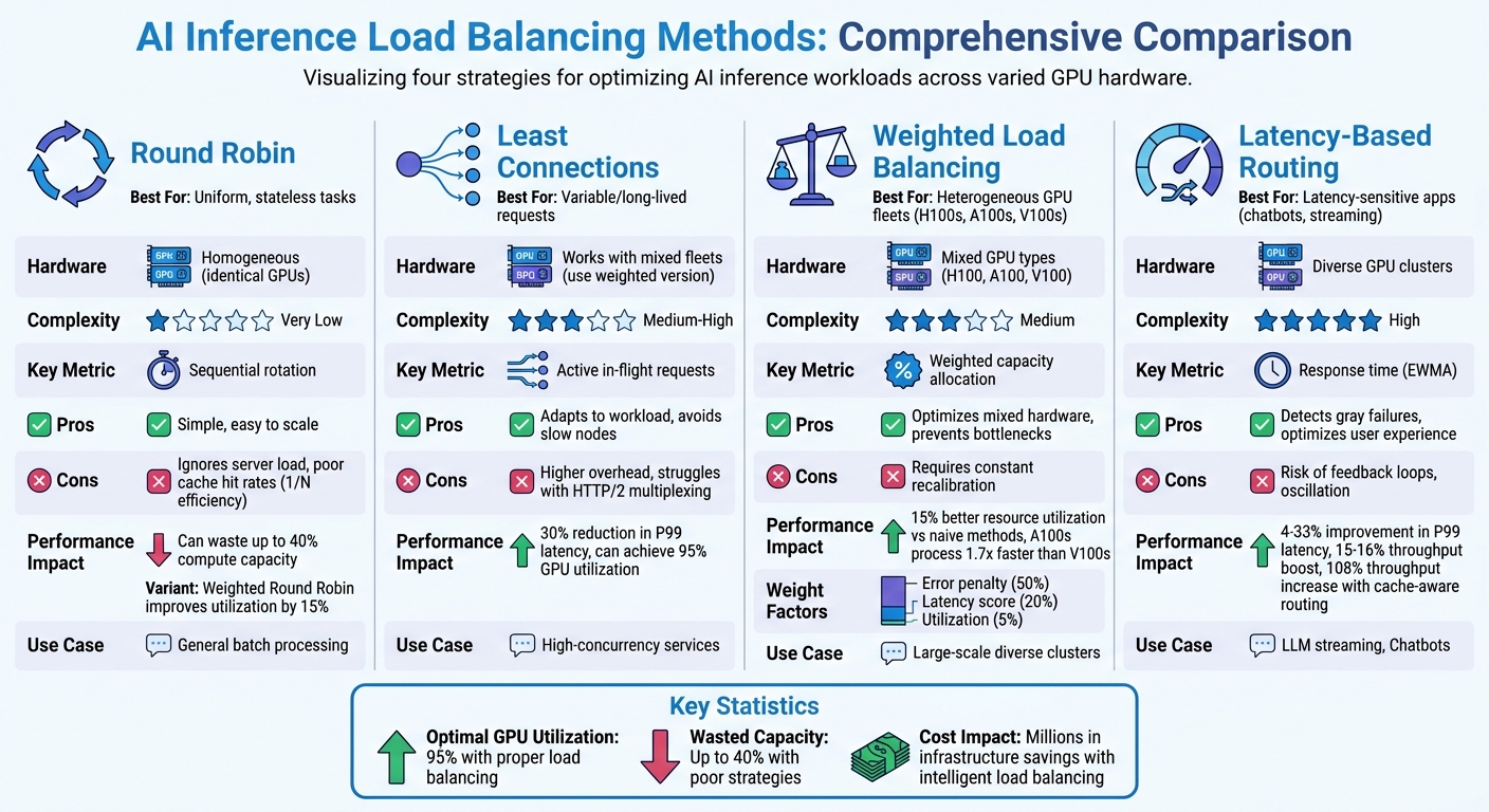
Load balancing for AI inference is critical to ensure efficient GPU utilization and minimize delays in processing requests. Unlike traditional web services, AI inference workloads are highly variable, requiring specialized strategies to distribute tasks effectively. Key methods include:
- Round Robin: Simple but struggles with uneven workloads and cache inefficiency.
- Least Connections: Dynamically assigns tasks to GPUs with fewer active connections, ideal for variable or long-lived requests.
- Weighted Load Balancing: Allocates traffic based on GPU capacity, optimizing performance in mixed hardware environments.
- Latency-Based Routing: Directs traffic to the fastest nodes, reducing delays and avoiding bottlenecks.
Each method has unique strengths and limitations. For example, weighted strategies improve resource use in heterogeneous GPU setups, while latency-based routing excels in reducing response times for latency-sensitive applications. Proper load balancing can push GPU utilization to 95%, significantly cutting infrastructure costs and enhancing performance.
AI Inference Load Balancing Methods Comparison Chart
Scalable AI Infrastructure: Caching, Load Balancing, and Inference at Scale | Uplatz

sbb-itb-bec6a7e
1. Round Robin
Round Robin (RR) is a simple and straightforward load balancing method. It works by sequentially distributing inference requests across GPU servers, using a counter to forward each request without maintaining any state.
One of the main benefits of Round Robin is its ease of scalability. Many modern systems include slow-start mechanisms to gradually ramp up traffic to new GPUs, allowing their caches to warm up before handling full loads. However, this simplicity can also be a drawback when dealing with the complex and varying demands of AI inference.
Challenges with Round Robin in AI Inference
The Round Robin method assumes all requests are the same, but in reality, processing times can vary significantly. For instance, a 10-token request and a 512-token request may be distributed consecutively, resulting in uneven workloads. Additionally, as the number of servers increases, the likelihood of hitting a server with the desired cache decreases, reducing cache efficiency to just 1/N.
Resource Utilization
Round Robin works well for homogeneous clusters where all GPUs are identical. However, in mixed fleets with GPUs of different generations, Weighted Round Robin (WRR) is a better choice. WRR allocates traffic based on each GPU's processing capacity. For example, an H100 GPU would receive more traffic than an A100 due to its higher performance.
Amazon SageMaker demonstrated the effectiveness of WRR in December 2025. By using weighted round-robin for multi-instance endpoints, they improved resource utilization by 15% compared to naive Round Robin when managing a fleet with heterogeneous hardware. In contrast, naive load balancing can waste up to 40% of available compute capacity.
Performance Metrics
Optimizing resource allocation directly impacts system throughput and reliability. Benchmarks from early 2026 showed that switching from standard Round Robin to cache-aware routing boosted throughput by 108% on similar hardware.
However, Round Robin has its risks. It doesn’t account for performance variations, so it may continue routing requests to servers that are slow but still online, leading to "gray failures". This can cause spikes in p99 latency, even when overall metrics appear normal. Pedro Ribeiro from Azion aptly summarized this limitation:
Round-robin is the default, not the decision.
Comparison: Naive vs. Weighted Round Robin
| Feature | Naive Round Robin | Weighted Round Robin |
|---|---|---|
| Hardware Suitability | Homogeneous (identical GPUs) | Heterogeneous (mixed GPU types) |
| Resource Utilization | Suboptimal for mixed fleets | 15% better than naive |
| Implementation Complexity | Very Low | Medium |
| Best Use Case | Predictable, uniform traffic | Scaling across different hardware tiers |
While Round Robin is simple and effective for uniform, predictable traffic, its limitations become evident when compared to more advanced methods like Least Connections or Latency-Based Routing.
2. Least Connections
Least Connections offers a more dynamic alternative to Round Robin by directing requests to the GPU with the fewest active connections. This method adjusts to the varying processing times often seen in AI inference, ensuring that tasks are sent to nodes that are genuinely ready for more work, rather than just following a fixed sequence.
How It Adapts
This algorithm shines in unpredictable workloads. For instance, when handling conversational AI or streaming large language model (LLM) responses via WebSockets, connection durations can vary significantly. Least Connections actively monitors ongoing sessions and diverts new requests from overloaded nodes. As Sanjay Singh puts it:
Least connections performs better than round robin in two common situations... long-lived connections... and variable request cost.
In mixed GPU setups, Weighted Least Connections becomes critical. For example, if you're working with a combination of H100s and A100s, assigning higher capacity weights to the more powerful GPUs ensures they handle a proportional share of the workload. This prevents slower GPUs from becoming bottlenecks.
Tracking Performance
The most important metric here is in-flight requests, not just the number of TCP connections. Modern protocols like HTTP/2 can handle multiple streams through a single connection, so relying on connection counts alone can be misleading. Tools like Kong Gateway v3.13+ now monitor in-flight requests to distribute traffic more effectively to backends with available capacity.
This method directly improves latency. For example, Microsoft Azure ML introduced response-time-aware routing based on Least Connections and achieved a 30% drop in P99 latency for inference workloads. Similarly, Anthropic uses a variation of this strategy - queue depth balancing - to maintain steady response times for their Claude model, even under fluctuating request loads.
Maximizing Resource Use
When implemented correctly, Least Connections can drive GPU utilization to 95%, while poor allocation could waste up to 40% of compute resources. By distributing tasks based on actual availability, the algorithm prevents overloading individual GPUs. Adding new GPU instances? Pair Least Connections with a slow-start mechanism to avoid overwhelming fresh nodes before their caches are ready. This approach sets the stage for more advanced techniques discussed later.
| Algorithm | Primary Signal | Workload Type | Adaptability | Overhead |
|---|---|---|---|---|
| Least Connections | Active in-flight requests | Variable/Long-lived requests | High; avoids slow nodes | Higher (requires state tracking) |
| Round Robin | Sequential rotation | Uniform/Stateless requests | Low; ignores server load | Minimal (stateless) |
| Weighted Least Conn. | Weighted in-flight requests | Heterogeneous GPU fleets | Very High | Higher (state + weight calibration) |
Next, we’ll dive into how weighted strategies can refine this approach even further.
3. Weighted Load Balancing
Weighted Load Balancing is a smarter way to handle non-uniform GPU fleets by distributing traffic based on each node's capacity. If you’re running a mix of H100s, A100s, and V100s, treating them equally isn’t efficient. Instead, this method allocates traffic proportionally, ensuring your most powerful GPUs handle more requests while slower hardware doesn’t drag down performance. By factoring in hardware differences and real-time performance data, weighted load balancing optimizes throughput across the board.
Scalability
One of the biggest perks here is scaling with mixed hardware. For example, an H100 might process twice the traffic of an A100 because it’s built to handle that load. This is especially useful for incremental scaling - you can add newer GPUs without being limited by older ones.
For providers of large language models (LLMs) managing multiple API keys, weighted balancing is a game-changer. It can distribute requests across keys with varying TPM (Tokens Per Minute) and RPM (Requests Per Minute) limits, helping teams bypass single-key bottlenecks. Additionally, slow-start mechanisms for new instances gradually ramp up their traffic share, avoiding overload during auto-scaling events. Modern systems even tweak weights dynamically to match real-time conditions.
Adaptability
Weighted systems today are highly dynamic. Automatic Target Weights (ATW), for instance, detect when a node has high error rates and temporarily reduce its traffic allocation. As the node stabilizes, its weight is gradually restored. These adjustments happen in real time, influenced by factors like throughput, latency, or health checks . Some systems update weights every 5 seconds to keep distributions finely tuned.
More advanced setups use multi-factor weighting. For example:
- 50% weight is tied to error penalties
- 20% weight reflects latency scores
- 5% weight accounts for current utilization
This approach avoids "gray failures", where a node might appear operational but performs poorly. By adjusting weights dynamically, resource usage stays efficient and balanced.
Resource Utilization
A key benefit of weighted balancing is avoiding bottlenecks caused by underperforming nodes. Traffic is matched to each GPU's VRAM and compute power, allowing for GPU utilization rates as high as 95%. Without proper balancing, up to 40% of compute capacity can go unused . For example, A100 GPUs process requests 1.7x faster than V100s, making proportional traffic distribution crucial for optimal performance.
Performance Metrics
Weights are typically calculated from factors like max_concurrent_requests, TPM/RPM limits, or hardware benchmarks . To maintain efficiency, monitor P95/P99 latency for each target to ensure high-capacity nodes aren’t experiencing spikes . Instead of just tracking connection counts, focus on queue depth and in-flight requests since inference processing times can vary significantly based on input sequence length. This level of monitoring ensures weights reflect actual performance, not just theoretical capabilities.
| Factor | Typical Impact | Purpose |
|---|---|---|
| Error Penalty | 50% | Reduces traffic to failing nodes |
| Latency Score | 20% | Penalizes nodes with slow responses |
| Utilization Score | 5% | Prevents overloading high-performing nodes |
| Momentum Bias | Additive | Speeds up recovery for stable nodes |
4. Latency-Based Routing
Latency-based routing ensures traffic is directed to the fastest-responding nodes by dynamically factoring in performance variations. This helps smooth out the impact of inconsistent processing times.
Scalability
This approach works particularly well for scaling diverse GPU clusters. In 2024, Amazon SageMaker tested the codegen2-7B model on ml.g5.24xl instances, scaling from 5 to 20 nodes. By switching from random routing to Least Outstanding Requests (LOR) - a latency-aware alternative - they achieved a 4–33% improvement in P99 latency and a 15–16% boost in throughput per instance. The router automatically adjusts for differences in GPU performance, such as when mixing A100s and V100s, ensuring traffic flows to the quickest nodes. This prevents bottlenecks at slower nodes and fine-tunes routing decisions to handle fluctuating workloads, building on traditional weight- and connection-based methods.
Adaptability
Latency-based routing isn’t just scalable - it’s also highly adaptable to changing system conditions. In real-world scenarios, GPUs can thermal throttle, cutting performance by up to 20%, networks can shift, and instances may degrade without fully failing. This method uses peak Exponentially Weighted Moving Average (EWMA) to track ongoing performance trends while ignoring outdated data. For example, if a node recovers from a slowdown, it can quickly rejoin the traffic pool. For generative AI workloads, which range from millisecond to multi-minute requests, this adaptability helps avoid the latency spikes that simpler algorithms struggle to manage.
Resource Utilization
By intelligently routing requests, GPU utilization can reach up to 95%. Continuous monitoring ensures that busy nodes don’t get overwhelmed while others sit idle, avoiding "hot partitions." In large-scale setups, even small efficiency gains can lead to meaningful cost reductions.
Performance Metrics
Key metrics for evaluating latency-based routing include Time to First Token (TTFT) for streaming applications, P99 end-to-end latency for reliability, and throughput per instance for efficiency. Using peak EWMA to measure latency across the entire process - from TCP connection to final response - provides a comprehensive view of performance. For traffic with sudden bursts, this approach can cut P95 latency by over 30%. Additionally, circuit breakers can temporarily remove endpoints exceeding failure thresholds, ensuring the router doesn’t favor nodes that appear "fast" simply because they are failing immediately. By balancing throughput and minimizing tail latency, latency-based routing effectively optimizes load distribution across diverse GPU clusters.
Advantages and Disadvantages
This section dives into the pros and cons of various load balancing strategies, summarizing how each approach influences the performance and efficiency of AI inference systems.
Every load balancing method has its strengths and weaknesses, which can significantly affect both system performance and cost. For instance, Round Robin is straightforward but overlooks the complexity of incoming requests, leading to reduced cache hit rates as the fleet size grows. As Mohammad Ashar Khan from DigitalOcean explains:
The cache hit rate that made caching attractive at one replica degrades almost linearly as your fleet expands.
Least Connections is better suited for handling variable workloads, as it directs traffic to the nodes with the fewest active connections. However, this method struggles in modern AI serving environments using HTTP/2 or HTTP/3, where a single connection can carry multiple streams with varying workloads. On the other hand, Weighted Load Balancing is critical for clusters with mixed GPU types. For example, A100 GPUs often process requests about 1.7 times faster than V100s in the same cluster. Still, it requires constant recalibration to account for dynamic factors like thermal throttling, which can cut performance by up to 20%.
Latency-Based Routing focuses on optimizing user experience by prioritizing speed and detecting "gray failures" - situations where a node is slow but not fully down. However, this method can create feedback loops, where failing nodes appear "fast" because they return error codes almost instantly. Pedro Ribeiro from Azion points out:
Round-robin assumes a world where every backend behaves the same, latency is stable, and 'healthy' also means 'fast enough.' Real systems aren't like that.
Here’s a quick comparison of the key advantages and drawbacks of each method:
| Algorithm | Best For | Key Disadvantage | AI Inference Impact |
|---|---|---|---|
| Round Robin | Uniform, stateless tasks | Ignores server load and request complexity | Poor GPU utilization; significantly lowers cache hit rates |
| Least Connections | Variable request durations | Tracking overhead; struggles with multiplexed HTTP/2 | Handles long-running generation tasks better |
| Weighted LB | Heterogeneous hardware (mixed GPUs) | Requires precise, ongoing weight calibration | Essential for clusters with mixed GPU generations |
| Latency-Based | Latency-sensitive apps (e.g., chatbots) | Risk of oscillation and feedback loops | Reduces TTFT; detects "gray failures" early |
The efficiency of load balancing has a direct impact on resource utilization. Proper allocation can push GPU usage to 95%, while poor strategies may waste up to 40% of compute capacity due to inefficient request distribution. For AI inference, Round Robin should be avoided for large language models (LLMs) unless tasks are strictly uniform and stateless; otherwise, it can cause significant tail latency issues. When scaling up with new GPU instances, consider a "slow-start" approach - gradually increasing traffic to allow for model loading, JIT/GC stabilization, and cache warming.
Conclusion
Choosing the right load balancing strategy depends on your workload and infrastructure needs. For simpler, uniform tasks, Round Robin might work, but for large language models (LLMs), more advanced methods are necessary. Least Connections is better suited for handling requests with varying durations, though it can falter when using HTTP/2 multiplexing. In setups with mixed GPU types, such as H100s and A100s, Weighted Load Balancing becomes critical to avoid bottlenecks caused by slower hardware. These considerations pave the way for strategies that significantly enhance performance.
For conversational AI and LLMs, cache-aware routing can improve throughput by as much as 108% compared to basic round-robin, while latency-based routing can cut P99 latency by 30% and help detect gray failures before they affect users. These improvements underscore the benefits of smarter routing.
As highlighted by the Introl Blog:
The difference between naive round-robin and intelligent load balancing translates to millions in infrastructure costs.
Efficient load balancing can push GPU utilization to 95%, while poor choices can waste up to 40% of compute capacity.
To optimize performance, businesses should align their load balancing strategies with their specific workloads and hardware setups. Start with weighted load balancing for environments with mixed hardware, incorporate Power of Two Choices (P2C) to handle traffic surges, and adopt cache-aware routing for scaling LLMs. Monitoring tail latency (P95/P99) and using slow-start policies during scaling are also crucial to avoid overwhelming new instances with cold caches.
FAQs
How do I choose the best load balancing method for my inference workload?
To pick the best load balancing method, aim for strategies that make the most of resources, cut down on latency, and prevent bottlenecks. Basic round-robin algorithms often fall short, leading to inefficiencies. Instead, consider advanced options like cache-aware routing, latency-based routing, or even AI-driven traffic steering. These methods can boost performance, reduce tail latency, and improve scalability. Always align your approach with the specific needs of your workload to get the best results.
What signals should my load balancer use for LLM inference: latency, in-flight requests, or queue depth?
To get the most out of LLM inference, it's crucial for your load balancer to focus on predicted latency signals. Today’s systems often lean on latency predictions for smarter routing decisions, rather than just looking at metrics like in-flight requests or queue depth. This shift allows for smoother scalability and improved efficiency when managing AI workloads.
How do I set and update weights for mixed GPU fleets without causing instability?
To maintain stability while updating weights in mixed GPU fleets, it's crucial to use adaptive load balancing. This approach dynamically adjusts weights based on real-time metrics such as error rates, latency, and throughput. These systems work asynchronously, recalculating weights every few seconds to ensure seamless transitions.
Additionally, incorporating health checks or circuit breakers can help. These mechanisms temporarily exclude underperforming nodes, ensuring that requests are distributed efficiently and the system remains stable during updates.