If I need a model I can explain line by line, I start with a tree. If I need more prediction power, I test C5.0 with boosting.
Here’s the short version: C4.5 and C5.0 are decision-tree methods for yes/no and category decisions like churn, fraud, and approval. They learn from past labeled data, split records into groups, and return a class prediction. C4.5 leans more toward clarity. C5.0 adds boosting and tighter pruning, which can improve results but can make the model harder to explain.
Before I use either one, I check 4 things:
- Use case fit - Is this a classification problem like churn, fraud, or lead conversion?
- Data fit - Do I have labeled history, clean features, and no future-data leakage?
- Model tradeoff - Do I want a single tree for auditability, or boosted trees for better performance?
- Validation fit - Am I reviewing precision, recall, F1, and segment-level results, not just accuracy?
A few points matter most:
- C4.5 and C5.0 do not prove cause - they find patterns
- Gain ratio helps stop bad splits on fields like IDs with many unique values
- Pruning helps cut noise and limit overfitting
- Boosting in C5.0 can fix prior errors across later trees
- Single trees can shift when training data changes
- Rare outcomes can fool accuracy - a model can look good and still miss many true positives
- Human review matters for high-stakes calls like lending, fraud, or customer treatment
Machine Learning | Decision Trees - ID3, C4.5, C5.0, CART, CHAID
sbb-itb-bec6a7e
Quick Comparison
| Criteria | C4.5 | C5.0 |
|---|---|---|
| Core method | Single decision tree | Decision tree with added options |
| Split rule | Gain ratio | Gain ratio |
| Main strength | Easier to inspect | Higher prediction power in many cases |
| Main tradeoff | Can overfit or shift with small data changes | Boosting can reduce clarity |
| Best fit | Audit-heavy cases | Cases where a single tree falls short |
| What I watch most | Pruning, leakage, class balance | Same checks, plus boosting complexity |
I’d sum it up like this: pick the simplest model that answers the business question, then pressure-test it on unseen data before deployment.
How a decision tree moves from data to action
From root node to leaf prediction
A decision tree turns labeled data into a prediction by making a series of splits, then following those splits to a final outcome.
It starts with a labeled question, like whether a customer will churn. Before the model begins splitting, raw fields are often turned into better predictors. For example, a last purchase date field can become days since last purchase. That gives the model something it can measure and compare in a direct way.
Next, the model looks at possible variables for the first split and chooses the one that cuts uncertainty the most. That split creates 2 or more branches. The model keeps repeating that step until another split adds little value or the node is too small to split with confidence. The last node in that path becomes a leaf and returns the class prediction, such as likely to churn.
When a new customer record enters the tree, it moves through the branch rules until it lands on a leaf. That leaf is the prediction.
Missing values don't automatically stop the process. If a value is missing, C4.5 spreads the record across branches based on the observed split probabilities. Instead of forcing the record down one path, the model weighs multiple paths by probability and still returns a prediction.
That split rule is also where C4.5 starts to behave differently from simpler trees.
Why gain ratio matters in C4.5
C4.5 uses gain ratio to decide which field to split on at each node. It adjusts information gain by factoring in how many branches a field creates.
Why does that matter? Because some fields can look stronger than they are. An ID number, for instance, might seem useful because it creates lots of tiny groups. But those groups usually don't help much when you apply the model to new data.
Gain ratio fixes that problem by penalizing fields that create too many small branches. So if an attribute produces dozens of narrow splits, it gets pushed down the list. The result is a fairer choice that leans toward predictors with more use.
Use the terms below as a quick reference while reading the rest of the guide.
Model-flow glossary table
| Technical Term | Plain-Language Meaning | Business Interpretation |
|---|---|---|
| Root Node | The first split in the tree. | The strongest factor driving the business outcome. |
| Branch | A path based on a specific data value. | A customer or event segment following a specific behavior. |
| Leaf | The final endpoint of a branch. | The model's prediction, such as Will Buy or Will Churn. |
| Gain Ratio | A normalized version of information gain. | A fairer split rule that is not skewed by fields with many unique values. |
C4.5 vs. C5.0: what changed and what to compare
C5.0 is basically C4.5 with extra horsepower. The split logic stays the same, but C5.0 adds boosting and stronger pruning. For most business teams, the choice comes down to this: do you want the cleanest audit trail, or do you want more predictive power? That’s the tradeoff.
What C4.5 does well
C4.5 works well for tabular business data when transparency matters more than squeezing out every last bit of accuracy. Its pruning step cuts back branches that don’t generalize well, which helps limit overfitting.
The big appeal is its path-by-path logic. You can follow how the model got to an answer, explain it to stakeholders, and defend it when someone asks, “Why did this case get that outcome?”
C5.0 keeps much of that readability, but once you lean on boosting, some of that clarity starts to fade.
What C5.0 adds in practice
C5.0 adds boosting to push accuracy and stability higher. The catch is simple: more performance often means less clarity.
Even then, results still depend on the basics:
- Data quality
- Class balance
- Feature design
- Validation setup
- Tool implementation
So C5.0 isn’t magic. If the data is messy or the setup is weak, boosting won’t fix that.
C4.5 vs. C5.0 side-by-side comparison
| Feature | C4.5 | C5.0 |
|---|---|---|
| Primary splitting approach | Gain ratio-based splits | Gain ratio-based splits |
| Pruning | Uses pruning to reduce overfitting | Improved pruning controls plus boosting |
| Boosting | Not available | Available; builds sequential weighted trees to correct prior errors |
| Interpretability | High; easy to audit and explain | High in single-tree mode; lower when boosting is used |
| Training speed | Faster as a single tree | Slower with boosting |
| Best use cases | Exploratory analysis and situations where explainability matters most | Cases where a single tree underperforms and accuracy matters more |
| Main risks | Can overfit noisy data and is less robust than ensemble methods | Boosting can reduce interpretability and adds complexity |
That tradeoff leads to the next question: when should you use trees instead of other predictive tools?
Strengths, limits, and when to choose trees over other predictive tools
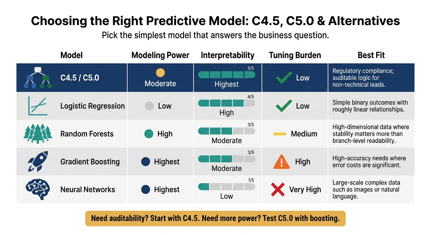
C4.5 vs C5.0 vs Other ML Models: Which Should You Choose?
Where C4.5 and C5.0 help and where caution is needed
The main question here is simple: is a tree the right model in the first place?
Use a decision tree when you need a model you can trace, explain, and defend. If a CFO, auditor, or regulator asks why a customer was flagged or why a loan was declined, a tree gives you a clear path to follow. That matters when auditability matters more than top-end accuracy.
Trees also need less preprocessing than many other models. If the business needs to move from raw data to a working model fast, that can be a big plus.
But single trees come with real weak spots. Small changes in the training data can reshape the tree, which makes them unstable [1]. They can also look good on rare outcomes while still missing most of the positive cases [5][4]. And if your inputs are correlated, the model can pull in old bias through proxy variables [3].
| Where C4.5 and C5.0 help | Where caution is needed |
|---|---|
| Auditable rules for approvals, declines, and exceptions | Instability: small data changes can reshape the tree [1] |
| Handling categorical and mixed data without heavy preprocessing | Overfitting: trees can fit noise unless pruned carefully [1] |
| Exploratory analysis to identify which variables drive outcomes | Class imbalance: rare outcomes can make accuracy misleading [5][4] |
| Generating readable if-then rules for operational workflows [4] | Data leakage: future information in training can inflate results [4] |
| Proxy risk: correlated features can hide bias [3] |
Those trade-offs decide whether a tree beats a simpler baseline or a stronger ensemble. Put bluntly: if you need a model people can inspect line by line, a tree is often a good fit. If you need the most stable or accurate result, it may not be.
How tree methods compare with logistic regression, random forests, gradient-boosted trees, and neural networks
Choose the model based on the decision you need to make - not on what sounds more advanced.
Logistic regression is often the best first model for simple binary outcomes when the relationships are roughly linear [2]. It is easy to explain and easy to maintain.
Random forests are more stable than a single tree. They build many trees in parallel and average the results, which cuts down the sensitivity problem [1]. You give up branch-by-branch readability, but you usually get a sturdier model.
Gradient-boosted trees, such as XGBoost or LightGBM, build trees one after another to correct prior errors. They often perform well on tabular business data, especially when accuracy matters a lot. The catch is the extra tuning work [5].
Neural networks sit at the other end of the spectrum. They can work well on large, messy datasets like images or text, but they are the hardest to explain. In regulated settings, that tuning burden and lack of clarity can be a serious issue [3].
| Model | Modeling Power | Interpretability | Tuning Burden | Best fit |
|---|---|---|---|---|
| C4.5 / C5.0 | Moderate | Highest | Low | Regulatory compliance; auditable logic for non-technical leads |
| Logistic Regression | Low | High | Low | Simple binary outcomes with roughly linear relationships |
| Random Forests | High | Moderate | Medium | High-dimensional data where stability matters more than branch-level readability |
| Gradient Boosting | Highest | Moderate | High | High-accuracy needs where error costs are significant |
| Neural Networks | Highest | Low | Very High | Large-scale, complex data such as images or natural language |
Validation, deployment, and next steps for business teams
Validation and deployment checklist
After you choose a tree model, test it on unseen data before you put it into production.
Start with one sentence. That sentence should state the decision, the target outcome, and the time window. If you can't say all 3 in one sentence, the project isn't ready to build.
Split the data into 3 groups: 70% for training, 15% for validation to tune the model, and 15% as a held-out test set used only for final testing [5]. If the data has a time dimension, use time-based validation. Train on earlier periods and test on later ones. Leave out future-state fields, like a cancellation flag that would not exist at prediction time.
Before deployment gets approved, check these controls:
| Check | What to confirm |
|---|---|
| Target definition | One-sentence goal with a measurable metric and time window |
| Data relevance | Training records match what the model will see in production |
| Leakage review | No future-state variables included in training features |
| Metrics beyond accuracy | Precision, recall, F1, and the confusion matrix are reviewed |
| Segment and bias checks | Performance and bias are tested across key customer or business segments |
| Pruning settings | Tree depth and pruning are reviewed to avoid overfitting |
| Error-cost trade-offs | False-positive and false-negative costs are documented per use case |
| Monitoring thresholds | Accuracy or drift thresholds are defined before deployment |
| Monitoring plan | Drift alerts and monthly performance reviews are scheduled |
| Human review | High-impact decisions have a human-in-the-loop step |
Error costs matter more than many teams expect. False positives and false negatives rarely cost the same. If you flag a loyal customer as likely to churn, you may waste a retention offer. If you miss a customer who is about to leave, you lose that revenue. Set the threshold only after you know which mistake hurts more.
Deployment isn't the finish line. It's the start of the monitoring cycle. Set a retraining schedule from day 1. Quarterly is a reasonable default, while fraud detection and e-commerce models may need updates more often [5][4]. Compare predictions with actual outcomes every month so you can catch accuracy decay before it starts distorting business decisions.
From model choice to tool adoption
Once the model is validated, move to the tools that support data prep, monitoring, and deployment. AI for Businesses is a curated directory of AI tools across marketing, sales, strategy, and management that teams can use to find and compare options.
Conclusion: start with the simplest model that answers the question
Start with the simplest model that can answer the business question. Then test it hard, monitor it closely, and move to more complex methods only when the evidence says you need to.
FAQs
When should I choose C4.5 over C5.0?
Choose C4.5 if you want a well-known decision tree method with plenty of documentation and a long track record. It works well for standard prediction tasks and gives you a solid starting point.
Choose C5.0 when speed, accuracy, and model size matter more. It usually performs better, runs faster, and builds smaller trees. C4.5 is a good baseline for exploratory analysis or simpler datasets, while C5.0 is a better fit for more complex, large-scale data.
How much data do I need for a reliable tree model?
Most predictive tools need 1,000 to 10,000 historical examples to produce decent accuracy. That’s the baseline.
But volume alone won’t save you. In most cases, you also need 6 to 12 months of clean, consistent, well-organized data to spot patterns and seasonality. If the data is messy, missing fields, or tracked in different ways over time, the model will struggle.
For use cases like demand forecasting, the bar is often higher. 12 to 24 months of history is commonly recommended so the system can pick up repeat buying patterns, calendar effects, and shifts across seasons.
The short version: data quality matters more than raw volume.
How do I know if boosting is worth the added complexity?
Boosting makes sense when prediction accuracy matters most and mistakes are costly.
It works by building trees one after another, with each new tree trying to fix the errors made by the earlier ones. That often leads to better performance than a single tree. The tradeoff is simple: boosting is harder to interpret than a method like CART.
Use it for high-stakes cases such as risk assessment or equipment failure prediction.
For exploratory analysis or simple, transparent decision-making, the extra complexity usually isn’t worth it.